200 tags at one row a second is 17.28 million rows a day, and at the 47 bytes a row that SQLite measured on this machine for a typed, indexed table, that is 814 MB a day and a 32 GB card full in 32 days. The same 200 tags logged on change, with a 0.5 % deadband on the fifty analogues and a heartbeat row every minute, come to about 28 MB a day and 10 GB for the year, with the ramps still recognisable in the trend. Nothing between those two PLC tag history numbers is a matter of taste; every term in them is either measured below or an assumption you can replace with your own count.
The answer, in the order it gets decided: the rate belongs to the tag, not to the logger; analogues get a deadband compared against the last written value plus a maximum interval; bools and counters are logged when they change; the row is typed and narrow and has no secondary index while it is being written; and the year is raw rows for the first ninety days and one-minute aggregates after that. The data logging article does the retention arithmetic for a SQL server with a disk array behind it. This is the same arithmetic for a card in a panel.
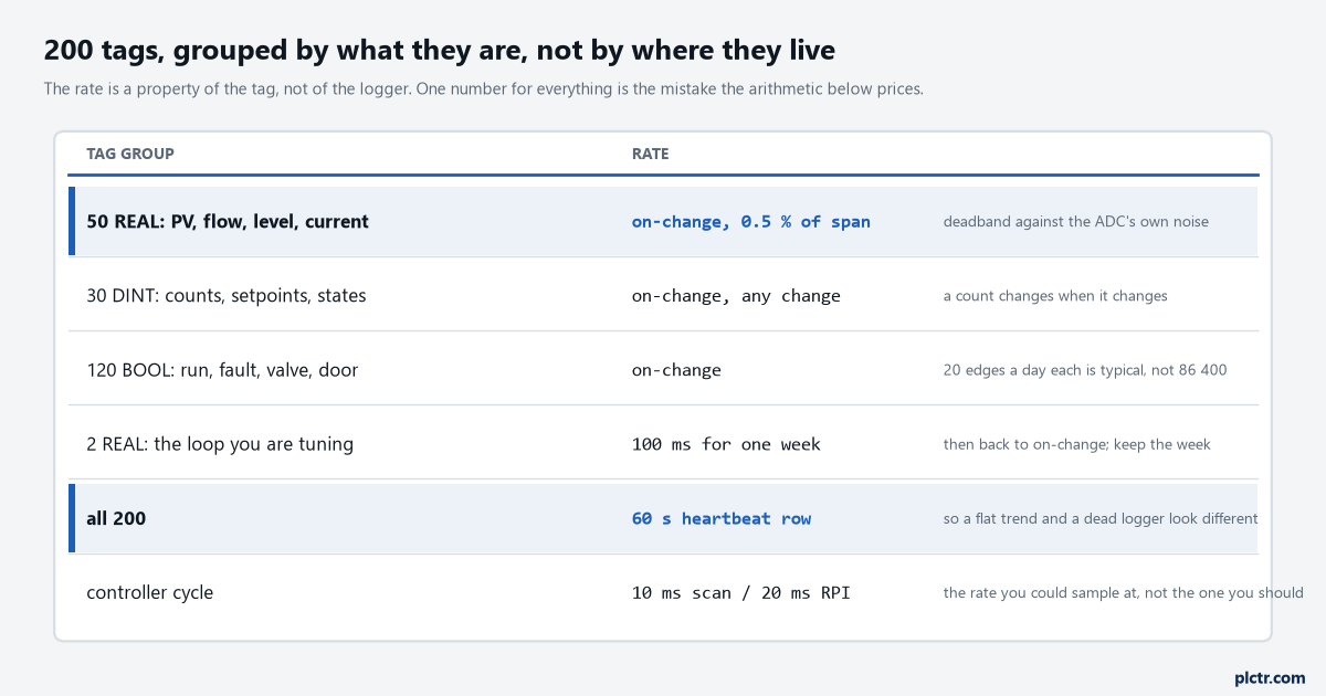
The controller’s 10 ms scan is the rate you could sample at. A tank level that moves 2 % an hour does not need it, and a PID loop you are tuning this week needs more than 1 s. One rate for all 200 is the mistake the arithmetic prices.
Where the PLC tag history rows come from
The rate is a property of the tag, and the first job is to stop treating “sample rate” as one setting.
Fifty of the 200 are analogues: process values, flows, levels, motor currents. Those are the tags with a shape worth keeping, and the shape is what deadband preserves. Thirty are DINTs: counters, setpoints, step numbers, state words. A count changes when it changes, and logging a state word every second produces 86 400 identical rows a day per tag until the one second it moves – so those are logged on any change, with no deadband at all. A hundred and twenty are BOOLs: run bits, faults, valve commands, door switches. A run bit on a machine that starts twenty times a shift produces perhaps sixty edges a day; a level switch that chatters produces sixty thousand, and that is a finding, not a logging problem. Two of the fifty analogues are the loop you are tuning this month, and for one week they earn 100 ms, which is where a PIDE bump test needs the resolution; when the week is over they go back to on-change and the week’s rows stay. And every tag, whatever its policy, gets a heartbeat: one row a minute regardless of change, so that a flat trend and a dead logger look different on the chart, and so that a query for “the value at 14:07” has a row within a minute of it. The one rate that is never right is the controller’s. A 5069-L306ER scans in a few milliseconds and a 1214C in ten; a Modbus meter answers as fast as you poll it. That is the rate the data could be read at and it has nothing to do with the rate it should be kept at. The pycomm3 and snap7 articles poll once a second and that is a good default for the read; what this page is about is what happens between the read and the INSERT
Deadband, on a signal
Compare against the last value you wrote, not the last value you read.
SPAN = {"Tank1_Level": 100.0, "Line4_Flow": 250.0}     # engineering units, from the scaling
DB_PCT = 0.005                                          # 0.5 % of span
MAX_GAP = 60.0                                          # heartbeat, seconds

last = {}                                               # tag -> (ts_written, value_written)

def keep(tag, ts, value):
    prev = last.get(tag)
    if prev is None or ts - prev[0] >= MAX_GAP or abs(value - prev[1]) >= DB_PCT * SPAN[tag]:
        last[tag] = (ts, value)
        return True
    return False
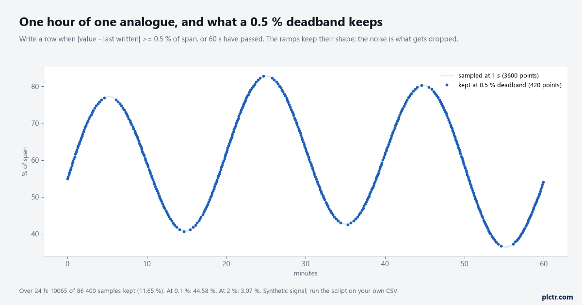
Synthetic: a 20-minute process cycle plus noise at the resolution of a 16-bit input. Over 24 h the 0.5 % deadband kept 11.65 % of the samples; 0.1 % kept 44.6 %; 2 % kept 3.1 %. Run the script on a CSV of your own tag before you pick the number.
The comparison against the last written value is the whole algorithm, and the version that compares against the last read value is the bug that costs a year of data. A tank filling at 0.3 % a minute, sampled once a second, moves 0.005 % between samples; against the last sample that is always inside the deadband, so the ramp is never written, and the trend shows the tank empty at 08:00 and full at 09:00 with nothing in between. Against the last written value the same ramp produces a row every 100 s, which reconstructs the ramp exactly. The number itself is set by the input, not by the process. A 16-bit card puts one bit at 0.0015 % of span and the analogue front end adds noise on top of that; 0.5 % of span is far enough above it that steady-state noise is dropped and small enough that a real 1 % move is caught within two rows. On the synthetic signal in the figure, which was built with noise at about that level, 0.5 % kept 11.65 % of the samples and 2 % kept 3 %; on a real 4-20 mA loop with a long cable the noise is larger and 0.5 % may still be inside it, which is why the caption says to run the script on your own data. Two things a deadband must not be allowed to do. It must not hide a step that mattered: a 0.4 % move on a value with an alarm limit at exactly that point is a move somebody will ask about, so for tags with alarm limits, set the deadband below the smallest limit hysteresis or log the alarm bit itself, which is a BOOL and is free. And it must not run on data with a regulatory purpose – a batch record, a sterilisation temperature, a custody-transfer flow. Those get logged at a fixed interval and kept, and the arithmetic for them is the 1 s column, and a card is the wrong place for them anyway.
The MAX_GAP
What a row costs, measured
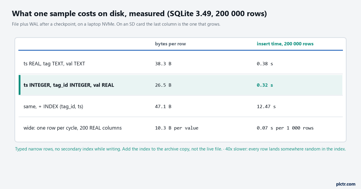
File plus WAL after a checkpoint, SQLite 3.49.1 on a laptop. The index column is the one to look at: on an SD card the 40x is the difference between a logger and a card that dies in a year.
Four tables, 200 000 rows each, and one index that changes everything about the card.
Each was inserted in batches of 200 with a commit per batch, in WAL mode, measured as file plus write-ahead log after a wal_checkpoint(TRUNCATE). The narrow table the queue article uses – ts REAL, tag TEXT, val TEXT – is 38.3 bytes a row, and that is with the tag name written out in every row. Typed – an integer millisecond timestamp, an integer tag id into a 200-row lookup table, a REAL value – is 26.5 bytes, a third less, and the queries get faster because comparisons are on integers. Add the index everybody adds, CREATE INDEX ON h(tag_id, ts), and the row is 47.1 bytes and the insert of 200 000 rows takes 12.5 s instead of 0.3 s. That is the number to stare at. The index is sorted by tag, the inserts arrive sorted by time, so every row lands in a different part of the index and every batch touches two hundred pages instead of one; on an NVMe that is 40x slower and on an SD card it is 40x slower and forty times the write amplification, which is how a card rated for years of sequential logging fails in one. Write the live file with no secondary index – the rowid primary key already keeps rows in time order, which is the order a trend asks for – and build the index on the archive copy once a day, after the rows have stopped arriving. The wide table, one row per cycle with 200 REAL columns, is 10.3 bytes a value and looks like the winner until the first tag is added, the first NULL has to mean “not sampled” rather than “sampled as nothing”, and the first on-change policy has to be expressed as a row where 199 columns did not change.
Storing the value as TEXT costs less than expected here – 12 bytes over typed – because SQLite stores short strings compactly. Where it costs is in every query that has to CAST before it can compare, and in the row where somebody logged '37.25 ' with a trailing space.
The year
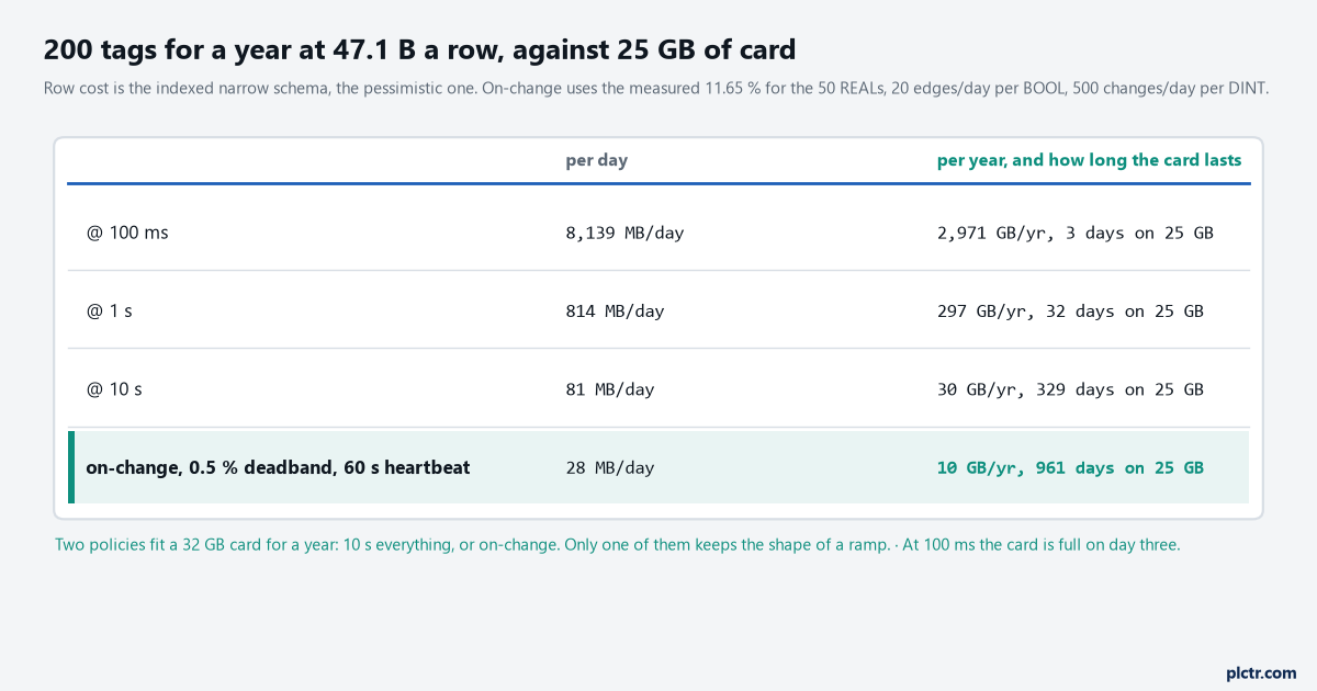
At 100 ms the card is full on day three. Two policies fit 25 GB for a year: 10 s for everything, or on-change with a deadband. Only the second keeps the shape of a ramp.
Rows per day is tags times samples per tag per day, and bytes is that times 47.
At 100 ms, 172.8 million rows and 8.1 GB a day, which is not a logging design, it is a fault. At 1 s, 17.3 million rows, 814 MB a day, 297 GB a year, 32 days on the 25 GB a 32 GB card has left after the OS. At 10 s, 81 MB a day and 329 days, so a year almost fits, and every ramp shorter than a minute is gone. On change, with the measured 11.65 % for the fifty analogues, fifty heartbeat rows a minute across them, 20 edges a day per BOOL and 500 changes a day per DINT – the last two are assumptions and yours will differ – 593 000 rows and 28 MB a day, 10 GB a year, and two and a half years on the card. The BOOL and DINT assumptions are the soft part of that number, and they are also the part you can count today: SELECT tag_id, count(*) FROM h WHERE ts > ? GROUP BY tag_id after one day of on-change logging tells you which twelve tags produce ninety per cent of the rows, and the answer is usually a chattering switch and a totaliser somebody logged raw. Then the year itself. Raw rows are worth keeping for as long as somebody will scroll a trend at full resolution, and ninety days is longer than anyone does; after that, one-minute aggregates – min, max, mean and last per tag per minute – are 288 000 rows a day for 200 tags, 13.5 MB, and 5 GB a year at the same 47 bytes, and they answer every question a monthly report asks. Delete the raw rows in blocks by ts, once a day, and know that the file does not shrink when you do: SQLite puts the freed pages on a free list and reuses them, so the file settles at its high-water mark, and VACUUM rewrites it smaller only when you ask, which on a card is a full copy of the file and not something to run from the poll loop.
The number the whole page turns on is 47 bytes, and it was measured on a laptop. Measure it on your Pi, on your card, with your schema, by inserting a day’s worth of rows and reading the file size; it will not be 47, and the difference is the card’s page size and the WAL’s share, and it is the first number in your own arithmetic.
Next step
Log everything on change for one day with the heartbeat on and no deadband on the analogues, then run the GROUP BY tag_id query and sort it. The top of that list is your sample-rate policy, written by the plant rather than by you: the tags that produce the rows are the ones that need a deadband or a rethink, and the tags that produce 1 440 rows a day are already at the heartbeat and need nothing. Set the deadband from a week of that tag’s own values, not from this page’s 0.5 %, and re-run the arithmetic with your own row cost. The timestamp article covers what ts should hold before any of these rows are worth keeping.