1200 tags collected once a second is 160,704,000 values a day, and at the 12 bytes a historian typically spends on a timestamp, a value and a status that is 1.93 GB a day and 704 GB a year. The same 1200 tags, with a deadband at the collector and a compression test at the archive, came out at 5,460,432 events a day and 23.9 GB a year in the run behind this page, which is a ratio of 29 to one.
Nothing in that ratio is free, and the whole of the cost is in what the second number threw away. A compression deviation of 0.80 A on a motor current with a 40 A span kept no archive point at all inside a real three-second event, and read it back as 0.03 A of noise. At 0.40 A the same event survived. That difference is the subject of this page.
The short version: the rate belongs to the tag, the deadband goes at the collector, the compression test goes at the archive, and the deviation is set from the signal’s own noise rather than from a percentage somebody liked.
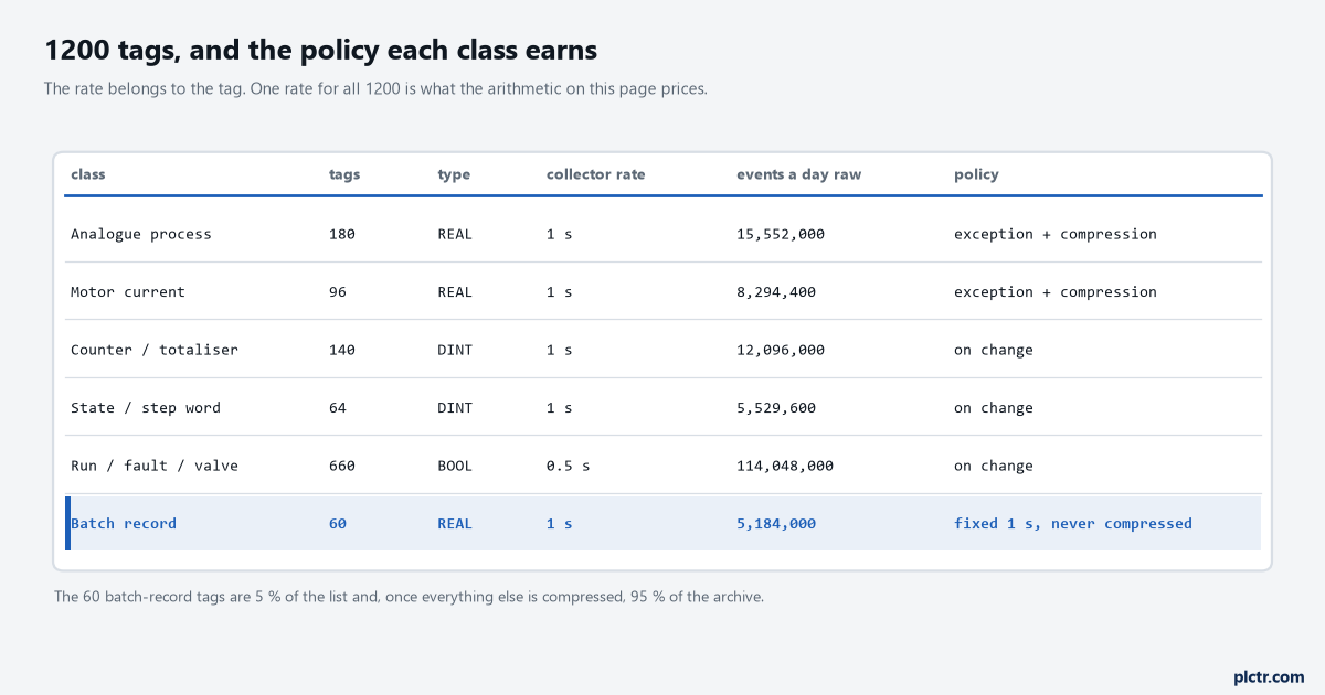
The highlighted row is 5 % of the tags. Once everything else on the list is compressed it is 95 % of the archive, which is the finding that decides how the disk is sized.
The arithmetic, before any settings are touched
Tags times rate times bytes times retention, and every term is yours to replace.
The list above is a real shape for a mid-sized packing plant: 276 analogues including motor currents, 204 integers that are counters and state words, 660 bools, and 60 tags that belong to a batch record. Collected flat at the rates shown, that is 160.7 million values a day. At 12 bytes an event it is 1.93 GB a day; written as 47-byte rows into SQL instead, which is what a typed indexed table measured on SQLite, it is 7.55 GB a day and 2.76 TB a year. The tag history sizing article does this same arithmetic for a card in a panel and measures that 47 bytes rather than assuming it; a plant historian on a server changes the storage numbers but not one step of the method.
Twelve bytes is the number to check on your own system before you trust anything below it.
Two filters, and they are not in the same place
One test decides what gets sent. A second, different test decides what gets kept, and they live on different machines.
The first is exception reporting and it runs at the collector — the OPC client, the interface, the edge node, whatever is actually polling the controller. Its job is to stop 86,400 nearly identical samples a day crossing the network for a tank that moved 2 % in an hour. OPC UA defines exactly this test in Part 4 as an AbsoluteDeadband on a monitored item, and the specification’s wording is worth having in front of you because it settles the argument that costs people a year of data: generate a notification if the absolute value of the last cached value minus the current value is greater than the deadband, where the last cached value is defined as the last value pushed to the queue. Against the last value pushed, not against the last value read. A tank filling at 0.3 % a minute moves 0.005 % between one-second samples, so compared against the previous sample it is always inside any sane deadband and the ramp is never sent at all; compared against the last value that went out, the same ramp produces a value every time it has genuinely moved. Part 4 adds two details the manuals gloss over. The deadband is ignored when the status of the item changes, so a tag going bad always reports regardless of the number you set. And for an array, the entire array is returned when any single element exceeds the deadband, which is how a UDT of thirty members turns into thirty times the traffic you budgeted for. Set the exception deadband low. Its purpose is network traffic, not storage, and anything it drops is gone before the archive ever sees it.
The second test is compression and it runs when the value reaches the archive.
Instead of comparing one value against one other value, it asks whether a straight line drawn between the archive points either side of this sample would land close enough to it. Two sloping limits open from the last archived point and narrow as each new sample arrives; while a line still exists that can reach every sample within the deviation, nothing is stored. When no such line is left, the previous sample becomes an archive point and the corridor reopens from there. The parameter names differ between products — check what yours calls the two deviations, because the collector one and the archive one are often spelled almost identically and confusing them is common — but the mechanism is the same everywhere, and so is the consequence: the error of what you read back is bounded by the deviation, not by the sample rate.
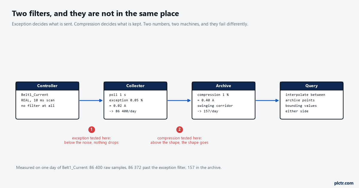
86,400 samples in, 157 archive points out, and the two numbers that did it sit on different machines. Neither one is a global setting.
The deviation is set by the noise, not by a percentage
Double one number and the storage changes by a factor of fifty. That is not a typo.
Belt1_Current in the run has a sample-to-sample noise sigma of 0.11 A on a 40 A span. At a compression deviation of 0.20 A — 0.5 % of span, the number people reach for first — the noise itself keeps breaking the corridor, and 8.96 % of the day’s samples end up in the archive, 7,744 of them. At 0.40 A, which is 1 % of span and about 3.6 sigma, the noise no longer reaches the limits and 157 points are kept. Same signal, same algorithm, one doubling, and a factor of 49 in what it costs to store a year of that tag. The lesson is not that 1 % is the right answer. It is that the useful setting sits a defined distance above the noise floor of that particular measurement, and the noise floor is something you can measure in ten minutes from a CSV of the tag. Take a day of samples from a period when the value was genuinely steady, take the standard deviation of the sample-to-sample differences and divide by the square root of two, and set the compression deviation at three to four times that. Below it, you are archiving noise at full rate and paying for it. Far above it, you are throwing away events. The other three shapes in the run behave differently for exactly this reason: a tank level with a slow sinusoid kept 0.61 % of its samples at 1 %, while a line speed that sits on a setpoint for hours kept nine points in the whole day, because nine points are genuinely all it takes to draw it.
Nine points for a day of a line speed is not a bug. It is the algorithm working.
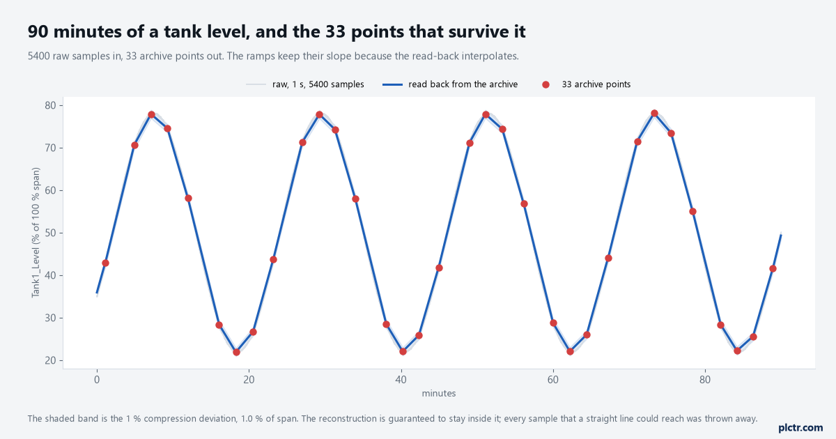
5400 samples in, 33 points out, and the ramps still have their slope. The shaded band is what the reconstruction is guaranteed to stay inside.
What the setting actually discards
A big event survives almost anything. A small one does not, and small ones are usually the interesting ones.
Two real excursions were put into the same motor-current tag. The first is a jam: the current goes from 18.4 A to a peak of 33.9 A for four seconds. That 15.5 A excursion was read back at its full depth at every deviation tested, up to 2.00 A, because an event that large breaks the corridor no matter how wide it is. The second is a gate sticking open: the current dips by 0.70 A for three seconds. At 0.20 A deviation the archive kept four points inside that window and read the dip back at 0.70 A. At 0.40 A it kept three and read 0.60 A. At 0.80 A it kept nothing inside the window, and the read-back shows 0.03 A — the event has not been blurred, it has been deleted. Nobody looking at that trend a week later has any way to know it happened. This is the part that gets left out of the sentence “the historian compresses the data”: what compression discards is bounded by the deviation, so any event whose amplitude is below the deviation can vanish completely, and the events that tell you a machine is drifting are almost always small. The rule that follows is specific rather than general. For every tag with an alarm limit on it, set the compression deviation below the smallest hysteresis band you alarm on, or accept that the archive cannot corroborate the alarm. And log the alarm bit itself as a separate tag, because a bool changing state costs one event and cannot be compressed away.
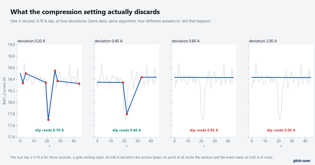
The two right-hand panels have no archive point inside the window at all. Same data, same algorithm, and two of these four answers to “did that happen” are wrong.
The read-back is interpolation, and that changes what a query means
Ask for the value at 14:07:03 and you are usually given a calculation, not a measurement.
A compressed archive stores the corners and nothing between them, so every point you did not store is reconstructed by drawing a line. OPC UA Part 11 is unusually honest about this: a raw history read returns bounding values on request, the values either side of the interval you asked for, so a client can draw the interval correctly. Part 4 goes further and puts the provenance in the status code itself. The HistorianBits, bits 0 to 4 of the DataValue InfoBits, are set only when reading historical data and say whether the value came back Raw, Calculated or Interpolated, with further bits for Partial, Extra Data and Multi Value. A client that ignores those five bits and prints the number as a measurement is the one that produces a report nobody can defend.
Two things follow that are worth checking in your own trend client.
Reading a compressed archive back with a held value rather than an interpolated one is wrong by a large margin. Held reconstruction error over the run’s day was between 30 and 80 % of span on every tag with a ramp in it, because holding the last archived value through a rise that the compression correctly summarised as two corners draws a staircase where there was a slope. The second is stranger and is the largest single error in the whole day. At a belt stop the true values run 18.44, 18.43, then −0.05 A on consecutive seconds. The archive kept the sample before the edge and the sample after it, and not the sample on it, so the read-back at that second is 9.2 A: a current the motor never drew, and a one-second stop that reads as a two-second ramp. Compression does not blur the value at an edge. It blurs the time of the edge by up to one collector sample, and if you are timing a stop to the second, that is the error to know about.
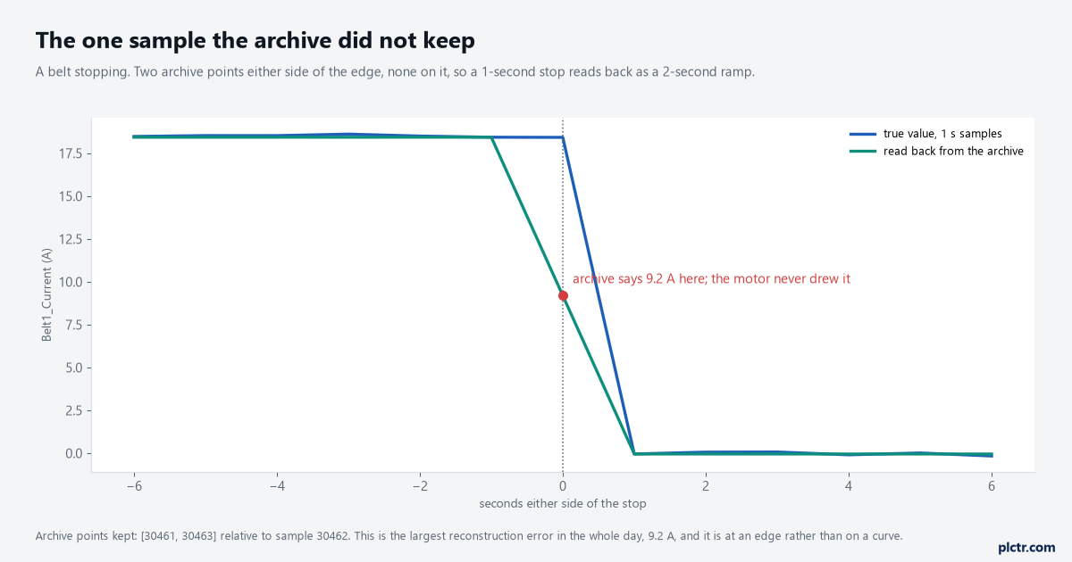
Two archive points either side of the edge, none on it. This is the largest reconstruction error in the whole day and it is at a corner, not on a curve.
The tags that must never be compressed
Four groups, and they will dominate your storage.
A batch record or a genealogy trace, a sterilisation temperature, a custody-transfer flow, anything an auditor will read: fixed interval, no deadband, no compression, and kept as raw values. A sequence-of-events record, where the whole point is the order and the millisecond. A counter or totaliser, which changes when it changes and whose intermediate values are meaningless. And any tag you are actively tuning this week, which earns a fast fixed rate for as long as the work lasts and goes back to normal afterwards. In the run, the 60 batch-record tags are 5 % of the tag list and, with everything else compressed, 5,184,000 of the 5,460,432 daily events — 95 % of the archive. The remaining 1140 tags come to 3.3 MB a day between them.
That is the number to take away. Sizing a historian is mostly an exercise in counting the tags you are not allowed to compress.
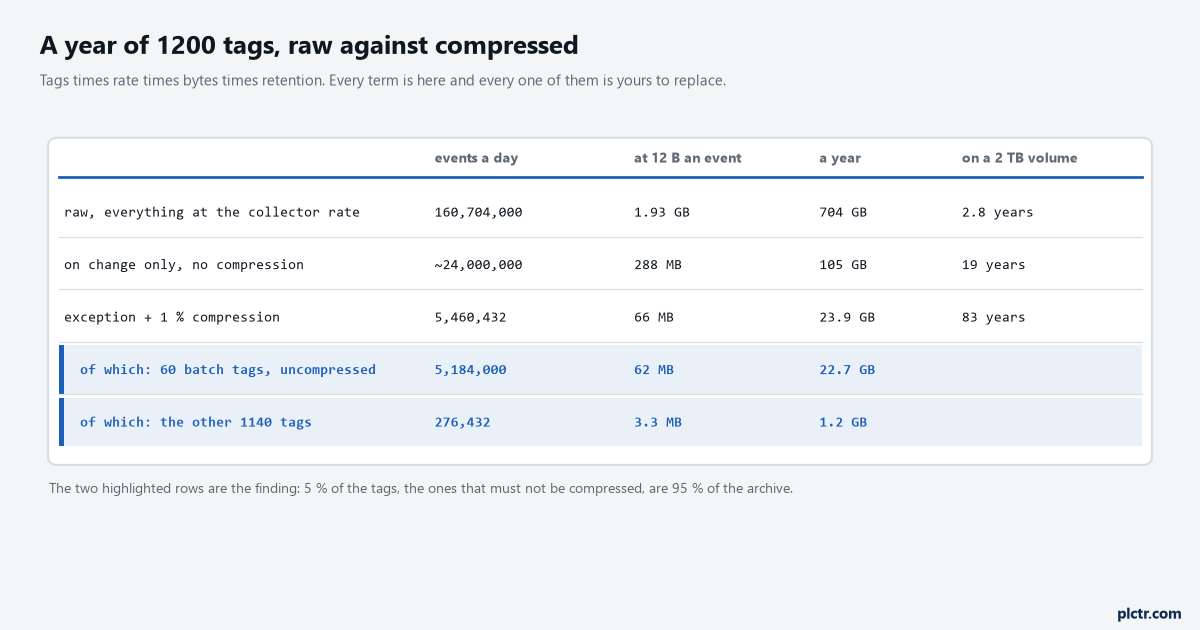
The last two rows split the compressed total. Sixty tags carry 22.7 GB of the year and the other 1140 carry 1.2 GB.
Next step
Take one week of one analogue tag out of whatever you have now, at full collector rate, as a CSV. Compute the sample-to-sample standard deviation over a period when the process was steady and divide by the square root of two: that is the noise floor, and three to four times it is your starting compression deviation for that tag. Then run the two events you care about through it — the smallest excursion anybody has ever asked you about, and a stop — and check that both survive the read-back at full depth. Do that for one tag from each class rather than all 1200, because the classes behave the same way within themselves and differently between. The timestamp article covers what has to be true of the clock before any of these rows are worth keeping, the database logging article covers retention once they are, and the trend page article covers what an operator is going to do with them. If the collector is OPC UA, the deadband and queue settings that feed all of this live on the monitored item, and the OPC UA tag to client path is where those are configured.